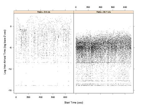
The left panel of the figure, an inter-arrival plot , displays the 2515 HTTP start times for one block, 7:45 a.m. to 8:00 a.m. on 12/11/98. Let s(k) for k = 1 to 2515 be the start times, and let t(k) = s(k) - s(k-1) for k = 2 to 2515 be the inter-arrival times. On the plot, l(k) = log base 2 t(k) is graphed against s(k). The log on the vertical scale is vital because inter-arrivals can vary over 16 powers of 2, a factor of about 64000, and small intervals are as important as large ones; so the vertical scale provides the requisite resolution to see this variation. The horizontal scale, however, conveys arrivals and inter-arrivals on the original scale. The connection rate over this block is 2.8 connections per second (c/s). The right panel of Figure 1 is an inter-arrival plot for the block 12:15 p.m. to 12:30 p.m. on the same day; the connection rate is 20.1 c/s.

Both panels show discreteness on the vertical scale, inter-arrivals piling up at a few values. This is a network effect, a small delay; each accumulation point is a time equal to the time it takes to process a packet in the network. For example, suppose two SYN packets are back to back, which happens a small fraction of the time. The inter-arrival time is the time it takes to read the first packet, which is the packet size times the wire speed; at the time of collection the speed was 10 megabits/sec.

Here is a collection of inter-arrival time plots (compressed postscript, pdf) used in the paper "On the Nonstationarity of Internet Traffic". Inter-arrival times of packets flowing from web servers to clients. Each page displays the packet inter-arrival times for one 5-minute interval. Due to large file size of the original plots, only a subset of 25 intervals out of 500 intervals is available for download here.