Doing science with prototype Virtual Observatory tools?
July 01, 2003
Bob Mann1,2 and Mark Allen3
1. Institute for Astronomy, University of Edinburgh (rgm@roe.ac.uk)
2. Professeur invité, Université Louis Pasteur, Strasbourg
3. Centre de Données astronomiques, Strasbourg (allen@astro.u-strasbg.fr)
1 Introduction
As the Virtual Observatory (VO) takes shape, it is vital that there is a closed feedback loop between
the developers of VO tools and the scientists who will use them, to ensure that the tools match the
scientific requirements of the astronomical community. With that in mind, we undertook an
exercise to see to what extent real science can be done with the existing first batch of VO prototype
tools, primarily the tools created for the AVO First Light Demo in January 2003. Our approach
was to take a science problem and to see if we could follow it through to the point of obtaining
scientific results using available tools, and identifying the problems that arose along the way. We describe the
results of this exercise in this note, and also supply the information required for other people to
reproduce what we did. We stress that our goal was to test the existing tools scientifically, but not
to do publication-quality science, so what follows does not include the same level of rigorous
checking that we would apply in our own research!
2 Available data and tools
The AVO First Light Demo focuses
on the manipulation of GOODS data using an
extended version of the Aladin image tool from
CDS, coupled with the Astronomy Catalogue Extractor
(ACE), which is a web service wrapper to the
SExtractor source extraction code.
The AVO demo version of Aladin includes a source tree of image data covering the GOODS Chandra Deep
Field South (CDFS) region, notably WFI (optical) and ISAAC (near-IR) data from
ESO, multi-epoch ACS optical data from the HST and X-ray data
from Chandra. Catalogues from these, and other data sets covering
this region, are included in this tree, via links to the VizieR
catalogue service at CDS. (These include a draft UBVRIJK catalogue created by the
EIS team from their WFI and SOFI data: this was kindly
made available for AVO development work by the EIS team, and should not be considered as being a
scientifically validated EIS data product at this stage.)
VizieR offers many formats for catalogue output, including
VOTable.
Attributes stored in VOTable files can be plotted using the
VOPlot tool developed by VO-India
project in collaboration with CDS. VOPlot can run as a standalone java application, or as an applet in a browser, and it has
been integrated with VizieR, so that plots can be generated directly as part of the catalogue search
procedure. Our exercise employed the publicly available VOPlot standalone version 1.0, and we note that
VOPlot is currently in an early development phase. In fact many changes were being implemented during the
running of this example, so the fixes implemented in the developmental June 12
version of VOPlot are noted. (Also a beta version of another tool,
TOPCAT, became available after
this exercise. We include a limited set of tests using TOPCAT in the
appendix)
One of the great advantages of using an XML-based data format, such as VOTable, is that
standard XSLT methods can be used to transform the data,
so that they can be read into analysis tools developed outwith astronomy. In what follows, we
give examples of using three such non-astronomical analysis tools:
Mirage, a "Java-based software tool for exploratory analysis and visualization of
classification and proximity structures of multi-dimensional numerical data" developed at Bell
Labs (and utilised in the NVO January demonstrations); Weka, a "machine learning workbench"
from the University of Waikato; and CViz, a
"visualization tool designed for analyzing high-dimensional data in large, complex data sets",
from IBM. Like VOPlot, all three of these tools are downloadable from the WWW as Java .jar files and are available
free for academic use (although CViz currently so only for a finite time period): this is surely
indicative of one future path of VO development, whereby astronomers can make use of applications
developed in other disciplines, with the task for the VO developers being how to integrate these tools
into their infrastructure, rather than developing bespoke astronomical applications themselves.
3 Example science topic: X-ray-detected EROs
Our testbed science problem follows the recent work of Roche, Almaini and Dunlop
(astro-ph/0303206), who have studied the
properties of Extremely Red Objects (EROs) in the GOODS CDFS field, as part of an on-going
investigation of a galaxy evolution scenario in which the stellar mass of large elliptical galaxies
seen at redshift zero is created in ultra-luminous dusty starbursts at high-redshift, like those
detected in the submm using
SCUBA,
and possibly later passing through an AGN phase.
One of the things that Roche et al. do to investigate this hypothesis is to seek associations
between EROs (defined to be galaxies with I-K > 3.75) and Chandra sources in the GOODS CDFS field, to
try and assess what fraction of EROs might contain obscured AGN, of the sort necessary to explain
the spectrum of the hard X-ray background. We repeat that aspect of their work as our testbed
science topic, seeking associations between the Chandra sources in the 1Ms CDFS catalogue of
Giacconi et al. (2002) and the draft EIS UBVRIJK catalogue. We then
investigate how the properties of those X-ray counterparts which are EROs compare with both the
remaining counterparts of the X-ray sources which are not EROs and the remaining EROs which are
not associated with X-ray sources. We also look for correlations between the X-ray and optical/NIR
properties of the X-ray-detected EROs, and seek further information about them from the ACS data of
the CDFS field.
4 Summary of the procedure followed in this exercise
In Figure 1 we show the layout of some of the datasets available in the CDFS field, using the
Aladin component of the AVO demonstration prototype.
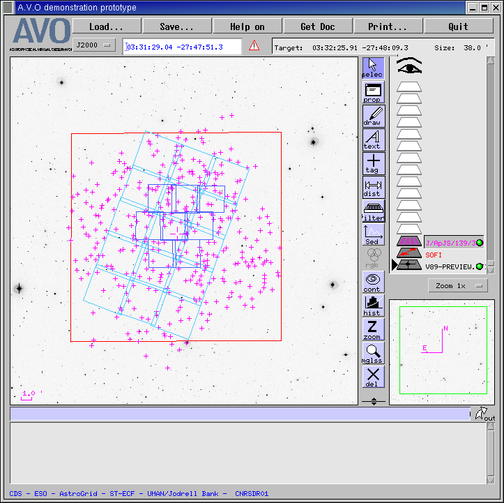
Figure 1. A summary plot of some of the data sets available in the CDFS area and used in this
exercise, namely: SOFI near-IR (red square), ISAAC near-IR (dark blues squares), first epoch
ACS (light blue squares), and Chandra sources (pink crosses), while the background image is a
WFI V band preview.
The background image is a WFI V band preview image (i.e. the pixels in the original image are
binned up to reduce the data volume) and the red square marks the boundary of the SOFI near-IR
data, so that the area within the red square is the coverage of the EIS UBVRIJK catalogue. For
comparison, the dark blue squares mark the area covered by the eight ISAAC fields used in the
creation of the ERO catalogue analysed by Roche et al., so we are considering a significantly
larger area of sky here. The pink crosses are the sources from the Chandra catalogue of Giacconi
et al., and the light blue squares plot the fields from the first epoch of ACS observations.
In outline, our exercise proceeds as follows. We start by investigating the selection of EROs from
the EIS UBVRIJK catalogue, by extracting a subset of the catalogue from VizieR in VOTable format
and reading it into both VOPlot and Mirage: VOPlot reads VOTables directly, while we have to run
an XSLT transform before reading the data into Mirage. We then perform the requisite I-K colour
cut in the tools and display the ERO sample that we have just created.
Having seen how to select EROs, we then cross-match the Chandra and EIS catalogues, in preparation
for investigating the properties of those associated sources which are EROs. Our cross-matching is
simply done on proximity, with a matching radius of 2 arcsec, following Roche et al., and
is performed within VizieR. Some manipulation in IDL is required to generate a VOTable containing
the combined X-ray and optical/near-IR attributes of the matched sources, and we assess the
validity of (a few of) these associations through the use of Aladin.
Our investigation into the properties of the X-ray-detected EROs then proceeds through the use
of VOPlot, Mirage, Weka and CViz. Each of these is designed to explore multi-variate datasets
like this, and we compare their performance in this task. This investigation identifies some
interesting sources, so we use Aladin and ACE to extract further information about them, using
one epoch of the ACS data in this field. Finally, we summarize our experience in undertaking this
exercise and draw some conclusions from it.
5 A detiled walk-through of the procedure followed
5.1 Selection of EROs from the EIS 7-colour catalogue
The draft EIS 7-colour catalogue was interrogated within VizieR, to select a subsample of galaxies
with K>17.5 (that marking roughly the brightest magnitude at which EROs are found) which was then
exported in VOTable format. We extracted a magnitude-limited
subsample of only 1000 sources, for our illustrative purposes: the VOTable for that subset is
availabe here. (Selection of larger samples is also
possible, taking into account the VizieR FAQ note for samples > 9999. ) We then sought to select
EROs from that sample, using both VOPlot and Mirage.
(It would be useful if VizieR could implement something analogous to "select
count(*)" in SQL so that you could find out how many entries satisfy
your selection criteria without having to extract them all, thereby
helping in the setting of appopriate criteria.)
VOPlot can, of course, be launched straight from VizieR, but we ran it in its standalone version,
loading the EIS subsample as a VOTable from disk, using VOPlot's simple Browse and Load
process. To aid ERO selection, we defined an additional I-K column in our dataset, making use of
VOPlot's Create new virtual columns mechanism, as shown in
Figure 2:
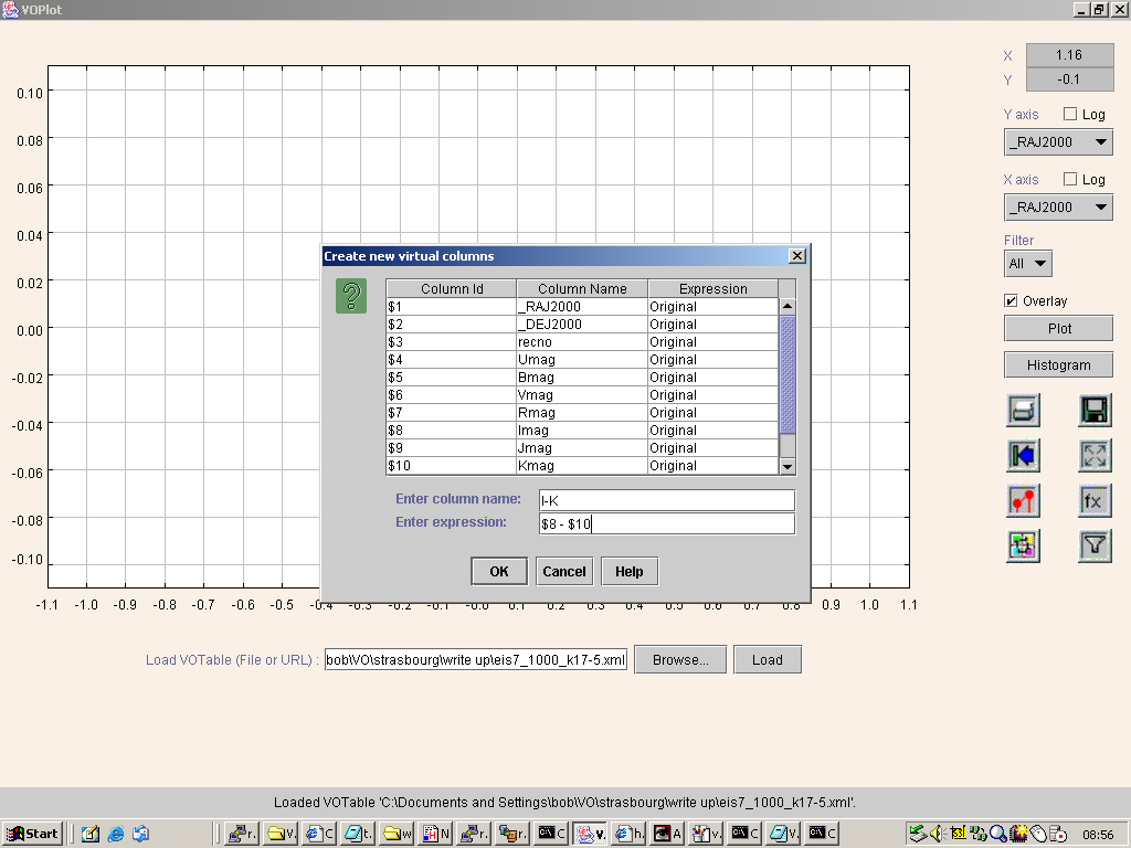
Figure 2. Defining a new virtual column in VOPlot.
This process is simply performed, with the additional column readily defined in terms of the existing
columns, through use of a set of basic mathematical functions. The Help pop-up lists a total
of 18 functions, including logarithmic and trigonometric functions, so there is significant flexibility
here, allowing both the investigation of positional properties and the creation of, say, optical/X-ray
flux ratios when the optical photometry is supplied in magnitudes.
We then performed the I-K>3.75 colour cut by defining a filter on our dataset, as shown
in Figure 3:
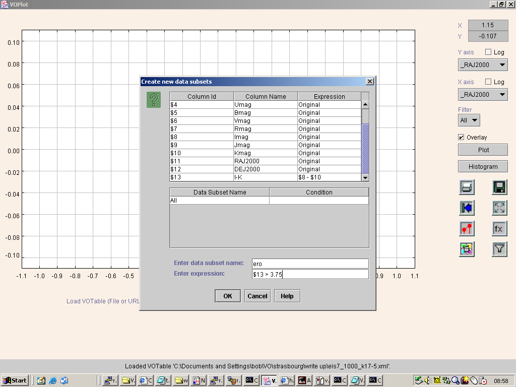
Figure 3. Defining a filter in VOPlot.
Again, this is simply done, using the Create new data subsets dialog box.
Armed with our named ero filter, we then sought to plot I-K against I for the full sample of
1000 sources, and overplot our ERO subsample in such a way that it stood out. This should be readily
done, since VOPlot has an Overlay option, which allows overplotting, and this can be used with
a named Filter, like our ero selection. In practice, the resulting plot, shown in
Figure 4
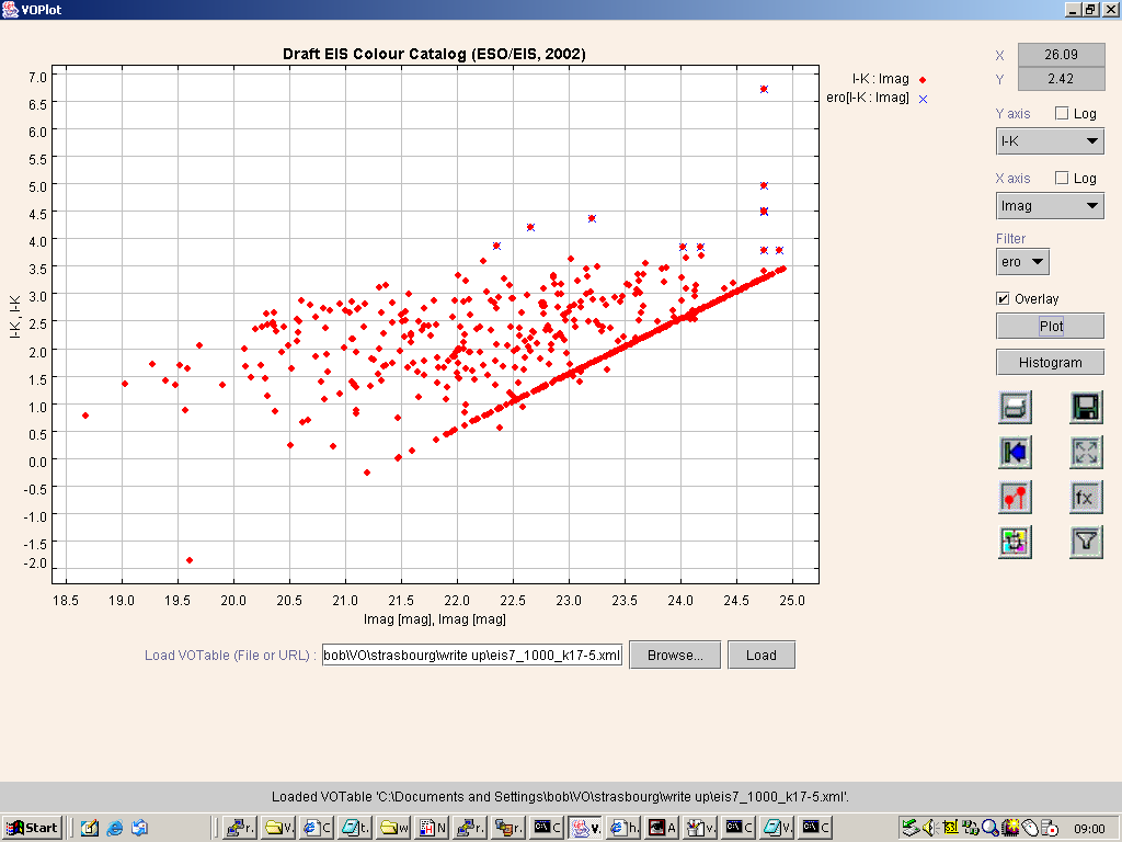
Figure 4. EROs selected from an (I-K) vs I colour-magnitude plot. Note the straight lines here
and in other plots are due to the magnitude limits of the catalogue.
was not as clear as we had hoped. The main and overlaid plots can be distinguished by plotting
symbols of different colour and/or shape. What we had wanted to do was to overlay our main plot
with red diamonds by the ERO sample in blue diamonds, but, while VOPlot did perform both those
operations, it then redrew the whole plot, as required to add notes of what the two symbols
denoted, and, in doing so, the blue diamonds became overplotted by the red diamonds, so that the
ERO subsample could not be distinguished. So, we had to resort to using blue crosses for the ERO
filter, since these could still be seen after the red diamonds were replotted, but this leads to
a somewhat unsatisfactory plot, as the ERO subsample does not readily stand out from the full
sample. Unfortunately the current VOPlot version lacks a mechanism for exporting
data manipulations made within the tool: in our example, it would be useful to be able to export
a VOTable which might have contained the additional I-K column, but certainly would have contained
an additional column which flagged the rows selected by our ero filter, ideally with the
filter definition being recorded in a human-readable form in the <DESCRIPTION>
element accompanying the <FIELD> element of the new column.
An analogous procedure can be followed in Mirage, once the data have been transformed into its
format. This transformation is aided by starting from an XML format, like VOTable, as all that is
required is the definition an XSL stylesheet expressing how the data are transformed and then a
standard XSLT engine can be used to performed the transformation. Ray Plante produced an
XSL stylesheet to convert from VOTable to Mirage format and posted it on the VOTable mailing list
some time ago: it is available there at
http://archives.us-vo.org/VOTable/0194.html. This needed to be modified slightly (changing
the name of one attribute to look for) for use with VOTables downloaded from VizieR: the revised
XSL stylesheet is available here. Armed with that stylesheet,
conversion of the data takes just a one-line call to an XSLT engine. We used the Java version of
Xalan, the free XSLT engine from
Apache, for which the one-line call is of the form:
java org.apache.xalan.xslt.Process -in temp.vot -xsl vot2mirage.xml -out temp.mirage
to convert VOTable temp.vot into Mirage-format file temp.mirage: the Mirage version
of the EIS subsample is available here. Mirage is launched
with a command like the following:
java -Xmx750000000 -jar Mirage0.2.jar -data temp.mirage
where the -X specifies that Mirage be allocated a larger amount of memory than it would be
assigned by default by the Java virtual machine.
Once the data file
has been loaded into Mirage, the user is first presented with a view of it in tabular form, as shown
in Figure 5:
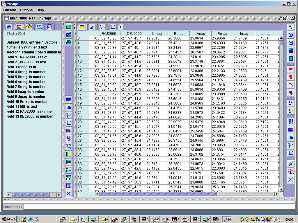
Figure 5. A table view of the data loaded into Mirage.
To define an extra column in Mirage to store the I-K colours, one does as shown in Figure 6,
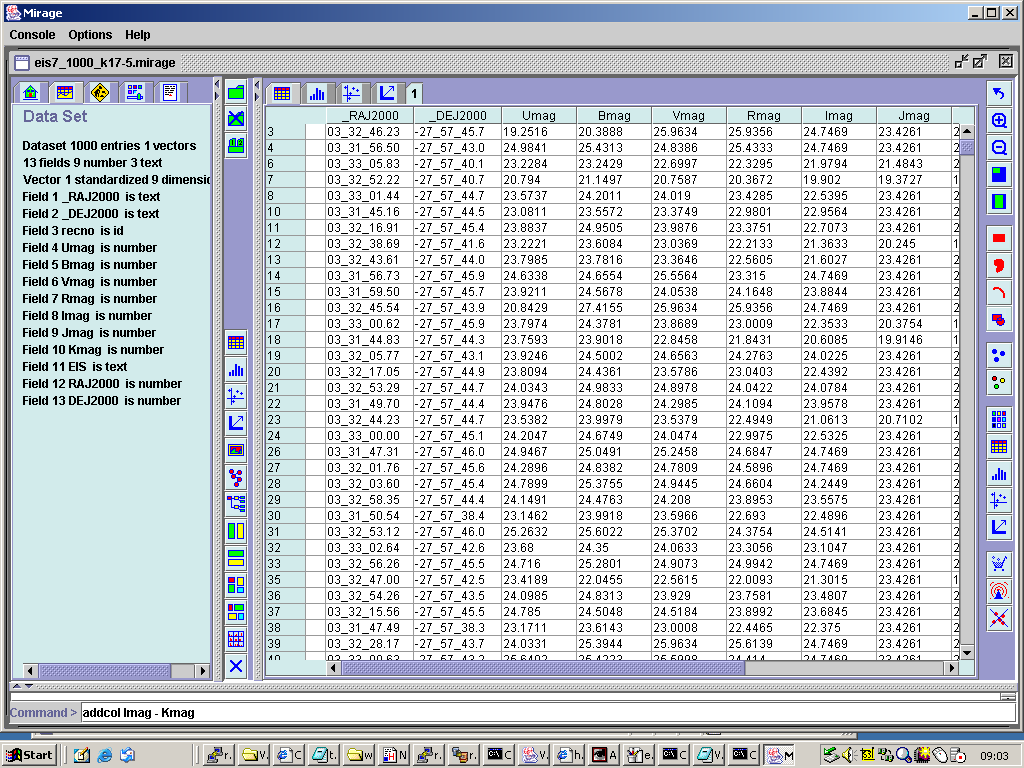
Figure 6. Defining an additional column in Mirage.
using the addcol command. This works for this case, but it is less flexible than the mechanism for
defining a new virtual column in VOPlot. One may only add a column which is the sum, difference or
product of existing columns, and there is no possibility of using a numerical value in the place
of the second column name: this restriction causes us a problem later, where we are not able to
rescale our X-ray fluxes so that their numerical values are large enough to be handled by Mirage's
axis-rescaling mechanisms. Mirage's selection mechanism is also somewhat less flexible than the filter
procedure in VOPlot. To perform our ERO selection we type select Imag-Kmag 3.75 10.0 at the
Mirage command line, since selections in Mirage have to be specified in terms of lower and upper
limits to the values in pre-existing columns. Note that, in VOPlot, we could have made our ERO
selection in one step, using a filter definition that included column numbers for both the I and
K band magnitudes, whereas, in Mirage, it has to be a two-step process, with the definition of an
extra column for I-K, followed by a selection of rows on the value in that new column.
Executing the select command in Mirage results in the highlighting of the rows in the table which
satisfy the selection criteria, as shown in Figure 7:
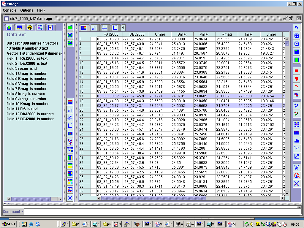 Figure 7. Highlighting in the data table view rows selected by a select command.
If the selection had been made while a scatter plot had been displayed, the rows in the table
satisfying the criterion would be overlaid, as shown for our EROs in an I-K vs I plot in
Figure 8.
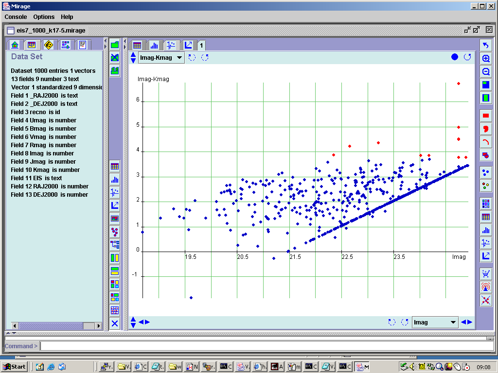
Figure 8. The ERO subsample in Mirage's I-K vs I colour-magnitude plot.
One of the neat things about Mirage is the way that a selection made in a plot making one sort of
presentation can be propagated through to other plots generated within Mirage. So, for example,
we could display a scatter plot of a different pair of attributes and the ERO points would continue
to be appear in a different colour. Selections can also be made graphically with Mirage, which makes
up for the lack of flexibility in the command line selection function: a rectangle or curve can
be drawn in an existing scatter plot to select data, or one can even "paint" an area of the plot
freehand, which would be very useful for selecting a cluster of points whose boundaries could not
easily be expressed in simple range cuts on attributes. Another advantage that Mirage has over
VOPlot is the ability to export data, so that we were able to write out, albeit into Mirage's own
ASCII data format, both the version of our EIS sample with the added I-K column and the ERO subsample
of that dataset.
5.2 Selection of counterparts to Chandra sources from the EIS catalogue
One of the biggest problems that we encountered in this exercise was the lack of a VO tool for the
generic cross-matching of catalogues which can deliver its results in VOTable format. Since we were
following the example of Roche et al. in making associations solely on the basis of proximity,
with a matching radius of 2 arcsec, we resorted to a slightly clunky method using VizieR. VizieR
is able to perform the matching of a list of targets, presented in Tab Separated Value (TSV) format in
a file, against the catalogue it contains. So, the first step in our selection of counterparts to
Chandra sources from the draft EIS catalogue was to extract from VizieR a TSV file containing the
positions of all the Chandra sources in the catalogue of Giacconi et al.. This we then
uploaded again into VizieR, using the List of Targets option, as described above and as shown
in Figure 9 below:

Figure 9. Loading the Chandra source list into VizieR to match against the EIS catalogue.
While multiple output formats are listed for VizieR's output from this procedure, only the
HTML table output worked perfectly, as shown in Figure 10
Figure 10. HTML table output from VizieR's cross-matching procedure.
Other output options generate "SIMBAD error" messages, are are currently not supported so we were
not able to extract what we desired, a VOTable containing the X-ray and optical/near-IR magnitudes
of the matched sources. In order to proceed with our exercise, we decided to create an ASCII file
from the HTML file shown in Figure 10 and use a small IDL
routine to match entries from it with entries in another ASCII file which contained the X-ray
attributes extracted from VizieR for the same set of Chandra sources. (For those wishing to
reproduce what we did, we provide the
IDL file, the matched source file
and the Chandra attribute file,
the matched source VOTable output file, and
the ERO subset VOTable, generated by including an
I-K>3.75 colour cut in the IDL routine: note
that the IDL code makes use of the readfmt routine from the
Astrolib library.) We could have performed the source
matching more easily using, for example, the
CURSA package from Starlink, but this
would not have returned results in VOTable format, which our quickly-written IDL code was able to.
No doubt the situation will change soon, as VOTable becomes more widely supported by astronomical
software packages, but this current lack of even a simple positional cross-matching tool that
returns a VOTable is a frustration.
(Re-attempting the matching procedure with VizieR, it was found that a cut down version of the
tab separated file, where only the coordinates were present, as opposed to the full version
returned by VizieR, could be used to obtain VOTable output of the matches. This VOTable
of cross matches is linked here. In principle this table could be converted
to a convenient format using an XSLT to generate the same result as done with the HTML table
and IDL script above.)
5.3 Validation of associations made between Chandra and EIS sources
Whilst we did not attempt as rigorous a validation of the associations we had made between the Chandra
and EIS sources as we would have in a real research project, we did check that the associations looked
sensible, by loading our VOTable of cross-matched source information into Aladin and overlaying the
error circles of the Chandra sources on an optical image of the region, marking the EIS catalogue
sources. Figure 11 shows part of the results of this:
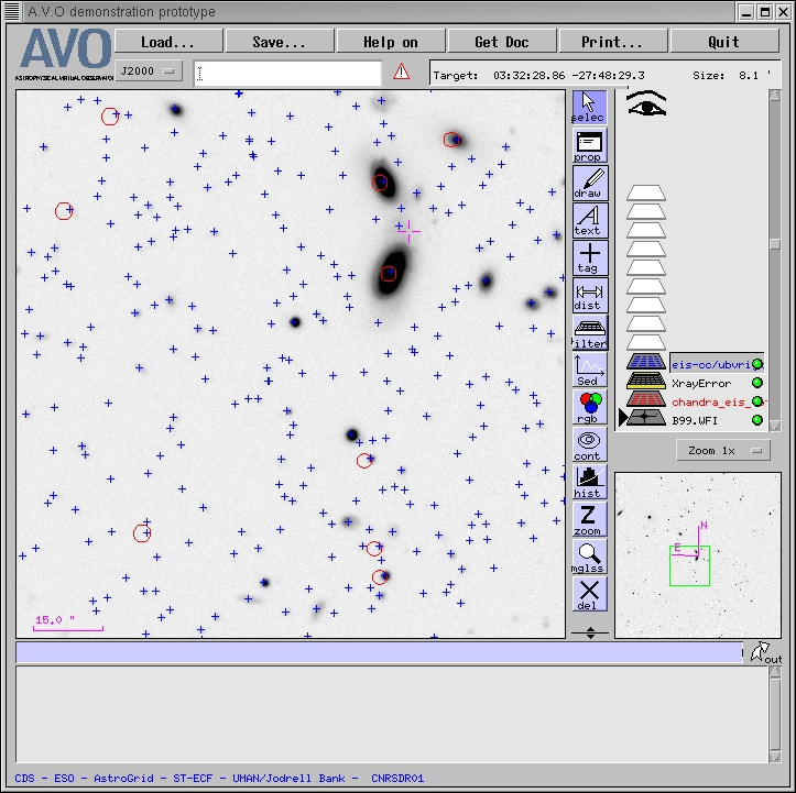
Figure 11. Chandra error circles (in red), plotted on an EIS/WFI B band images, with the
positions of the EIS catalogue sources marked as blue crosses: note the apparent offset in the
astrometric reference frames of the Chandra and EIS data.
The error circles in Figure 11 were created using Aladin's filter mechanism, which allows
us to define the size
of the circle to be drawn at each Chandra source position by using the values in the PosErr
column of our cross-match VOTable, which records the uncertainties in the Chandra source positions
listed in the Giacconi et al. catalogue. Figure 12 shows how this filter was defined in
Aladin.
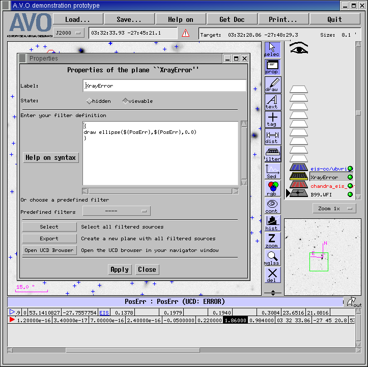
Figure 12. Defining a filter in Aladin, so that it will plot the error circles for all
the Chandra sources.
The two bright galaxies in Figure 11 intrigued us, so we selected cutouts from three of the
ACS frames in this field (F435W, F775W, F850LP) and created an RGB image from them in Aladin,
on top of which we overlaid the Chandra error ellipses again and the positions of EIS catalogue
sources. The result is shown in Figure 13:
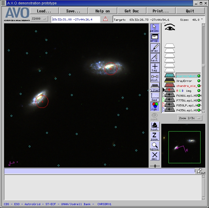
Figure 13a. Zooming in on two of the Chandra/EIS associations; overlaying Chandra error circles
(red) and EIS catalogue source positions (blue diamonds) on an RGB image created by Aladin from
the F435W, F775W and F850LP ACS images of this field.
The AVO prototype also allows an SED of catalog data to be plotted. This is shown in figure 13b.
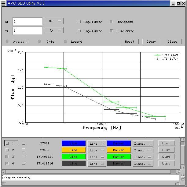
Figure 13b. SED of selected EROs.
Figure 11 indicates an apparent offset in the astrometric reference frames of the Chandra and EIS
datasets. We tried to investigate this more thoroughly, by looking at the distribution of offsets
between the matched X-ray and EIS source positions in the (RA,Dec) plane, but this proved impossible
with the current versions of VOPlot and Mirage. VOplot 1.0 seems unable to handle RAs and Decs in
decimal degrees. A developmental unreleased version of VOplot did however fix this problem,
and allowed construction and plotting of columns of RA and Dec offsets, see Figure 13c.
Figure 13c. Positional offsets between the Chandra and EIS datasets.
As noted above, Mirage allows the creation of a new column using only the
sum, difference or product of two existing columns. This means that it is not possible
to compute in Mirage a column to store the angular positional offsets in the RA and Dec directions
in arcsec, which is really what is wanted. In the light of that, it was decided just to compute the
difference between the RAs and Decs directly, neglecting the cos(dec) term for the angular distance
in the RA direction and keeping the results in degrees, since that's what the original columns
are in. Clearly, this resulted in very small numbers (of order 10-4 or
10-5), and it proved
impossible to get Mirage to plot these values on a graph with sensibly-scaled axes - and the
absence of a means of generating a new column by scaling the data values meant that it proved
impossible to produce a useful plot of the distribution of positional offsets in Mirage, either.
5.4 Investigating the properties of X-ray detected EROs
In this section we describe our investigation of the properties of the X-ray detected EROs with
the various tools described in Section 2 above. Our goal was to see how their properties compared
with those of two other populations, the non-ERO counterparts for Chandra sources from the EIS
catalogue, and the remaining EROs from the EIS catalogue which are not associated with Chandra
sources.
5.4.1 VOPlot
VOPlot 1.0 had some problems loading the VOTable file containing the matched source information that
we generated with our IDL routine. It seemed unable to match up some of the <FIELD> elements
defining table columns with the appropriate column of data extracted from the <TABLEDATA>
element. This is illustrated in Figure 14
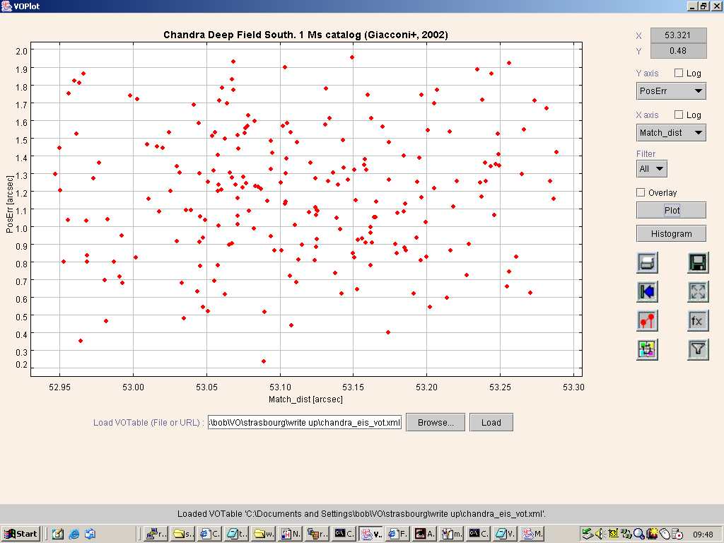
Figure 14. Illustrating the column mismatch in VOPlot resulting from loading our VOTable:
the axes say that this is a plot of PosErr against Match_dist, but the data
values plotted are for Match_dist against EIS_RAJ2000.
which shows a plot labeled as being PosErr against Match_dist. In fact, the values
plotted as being PosErr are, in fact, the values of Match_dist, the next column in
the table, while those purporting to be Match_dist are actually those of EIS_RAJ2000
which is the column which follows it in the table. Also, trying to plot the Kmag column causes
an ArrayIndexOutOfBoundsException to be thrown by VOPlot and the program
was unable to display that plot. We have not tracked down the cause of this
problem, but it does appear to be a problem with VOPlot and not with our VOTable: we checked that
our file was a valid VOTable document by validating it against the VOTable schema, using the Java
version of the Apache parser, Xerces, and
the XSLT-transformed version of the data loaded into Mirage has no such mismatch between column
titles and values. ( Subsequent tests with the developmental version of VOPlot show this bug
to have been fixed)
Despite this, we were able to identify which column stored in VOPlot corresponded to
which column in the VOTable, by comparing plots made with VOPlot and Mirage, and we were able to
create new columns with names matching the correct columns of data values. This did not work
completely, however, as we wanted to create a Total (0.5-10.0keV) X-ray flux, by adding the soft
and hard band fluxes from the Chandra catalogue, but an exception was thrown when parsing the
expression to set this up. This error seems to be present in both VOPlot 1.0 (where account of the
row mis-labeling is taken into account), and with the developmental VOPlot.
Figure 15 shows one interesting plot that did result from our investigation with VOPlot using the
columns already present in the table:
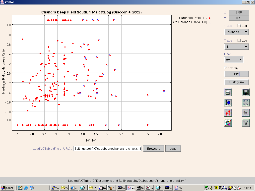
Figure 15. Hardness ratio against I-K colour for the Chandra-EIS associations by VOPlot.
This plots X-ray hardness ratio, HR> (defined to be HR=(H-S)/(H+S), where H
and S are, respectively, the hard and soft band X-ray fluxes), against I-K colour,
for all Chandra sources associated with EIS objects (red diamonds) and for the ERO subset (blue
crosses underneath red diamonds). It is interesting to note that ERO counterparts are found across
the full range of HR, implying that a number must harbour AGN, since passive ellipticals and
dusty starbursts alone should be soft X-ray sources. A second noteworthy point is the hint of a
difference in the I-K colour distribution as a function of HR for the ERO subsample.
It appears that the harder EROs, with HR-0.4 occupy a narrower range of I-K space
than the softer subsample.
5.4.2 Mirage
Similar procedures can be followed in Mirage. In Figure 16 we plot our analogue of Figure 15 from
Roche et al., which plots the X-ray hardness ratio against total (0.5-10.0 keV) X-ray flux.
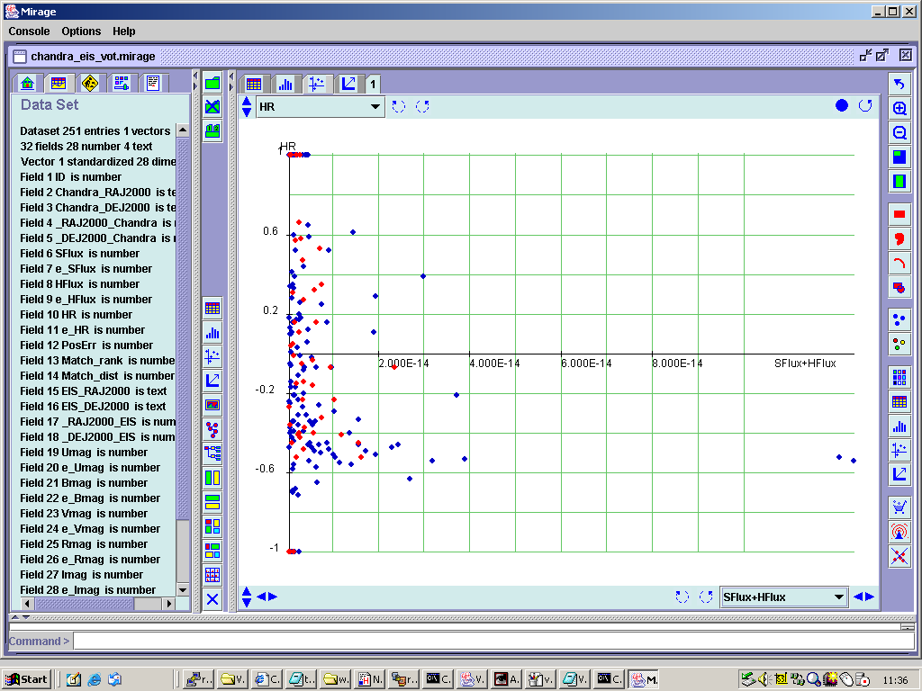
Figure 16. Hardness ratio against total (0.5-10.0 keV) X-ray flux for all the Chandra/EIS
associations (blue), with the ERO subsample overlaid in red.
A problem with this plot results from the small numerical values of the X-ray fluxes
(10-16 to 10-14 erg/s/cm2),
which are too small for Mirage's
axis rescaling procedure to work. Also, Mirage does not offer the capability of making logarithmic
plots (although it does permit the input of externally generated columns with
"addcolfrom" function). VOplot does allow logarithmic axes, by either the "log"
checkbox next to the axis selection menus, and also by definition of new virtual columns using logarithm function.
A benefit of using Mirage is the ability to work on multiple windows (plots) at the same time,
with the concept of projecting selected subsets of data to the various plots.
5.4.3 Weka
We briefly investigated the exploration of our matched Chandra/EIS source list using Weka, which
is a suite of data mining algorithms. Weka has its own data format, but our VOTable was readily
converted to that format using a XSL stylesheet, which we make available
here and which was created from the stylesheet for VOTable-to-Mirage
transformation via a few modifications. We ran Xalan to perform the tranformation, as before,
(yielding this ARFF file) which was loaded into Weka, which had
been launched with the command java -jar weka.jar: Figure 17 shows the result of this
procedure.
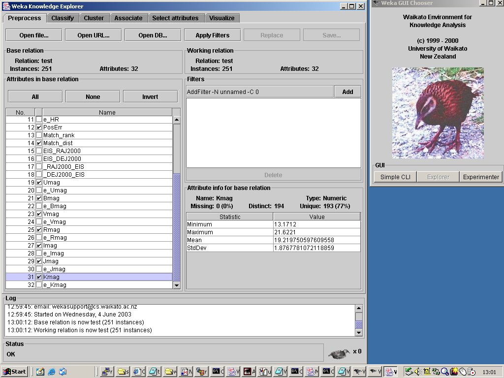
Figure 17. The Chandra/EIS dataset loaded into Weka, and with the attribute to be used in the
clustering procedure selected.
Launching Weka brings up the Weka GUI Chooser, shown on the right, from which we have chosen
the Weka Knowledge Explorer, on the left. We have loaded into that our dataset, and have
selected a subset of attributes to study by the use of the check-boxes in the Preprocess
pane. Note that statistical information about an attribute selected in the left hand pane is
presented on the lower right hand pane. Our intention in loading the Chandra/EIS data into Weka
was to use some of its clustering tools to see whether we could detect different populations in the
multi-dimensional space defined by the nine band X-ray and optical/NIR photometry data we have for
these sources. As an initial attempt at that, we just clicked on the Cluster tab in the
Explorer window, which provided us with the means of launching one of Weka's clustering
algorithms, details of which are given in the
Weka book. We chose the default
clustering algorithm, EM, with its default set of parameters, and chose to run it using 66% of
our data as a training set. That yielded the following results pane:
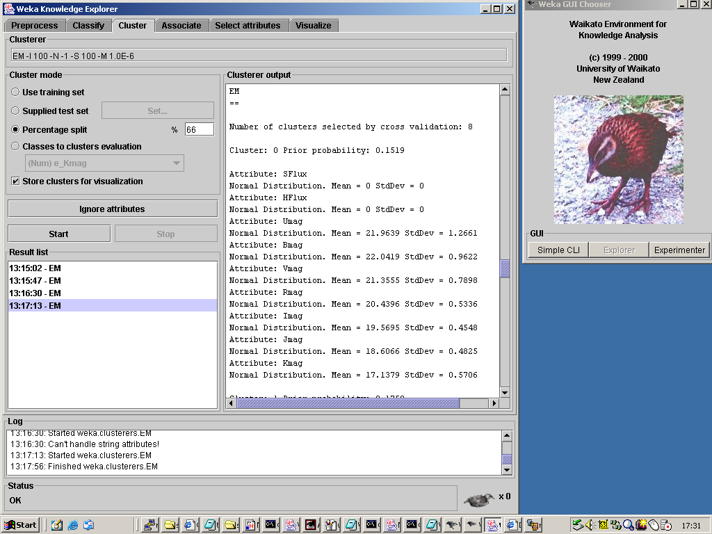
Figure 18. The result of running Weka's default clustering algorithm (EM) on the 9-dimensional
photometric data space created from the Chandra/EIS dataset.
Running the EM algorithm in this way on the 9-dimensional photometric space yields a set of nine
clusters, but upon closer inspection of the results, two things become clear. Firstly, the two
X-ray fluxes have effectively been ignored, since the clustering algorithm took their numerical
values (10-16 to 10-14, in
erg/s/cm2 recall) to be directly
comparable to the optical magnitudes, so that the, essentially, all the sources had the same
X-ray fluxes, so that the two fluxes would not distinguish between sources in their assignment to
clusters. The second thing to note is that, if one ranks the nine clusters in order by
the mean value of the magnitude of the cluster members in a particular optical band, then the
ranking is almost identical across the seven optical/near-IR bands. This indicates that the spread
in source colours is much smaller than the spread in source magnitudes - i.e. to lowest order, all
sources have the same SED, and all that differs between them is an overall scaling in magnitude.
This is clearly not the result that we wanted to get from this exercise! The data space within which
we should have sought clusters would have been one spanned by flux ratios, rather than fluxes, so that
we found sets of source with different SED type, and with those fluxes normalised so that all of them
would have similar weight in assigning cluster membership. Since Weka is intended to be an
extensible data mining framework, rather than a comprehensive standalone tool, it does not provide
many filters, such as we could use to perform this normalization, but, rather, it provides a
mechanism whereby users can write small java classes to implement filters and have them run in Weka.
Weka's Select attributes tab calls up algorithms to select the most discriminating attributes:
for example, if we had run that with our input dataset, it would have eliminated the two X-ray fluxes.
This would be a useful preprocessing step if we had normalised our data before loading them, since it
probably would have reduced the dimensionality of the problem - and, hence, the time taken to run
the clustering algorithm - by noting that the set of seven optical/near-IR magnitudes contain some
redundancy, given that the spread of colours in the sample is smaller than the spread of magnitudes.
Weka has its own visualization capabilities, as illustrated in Figure 19:
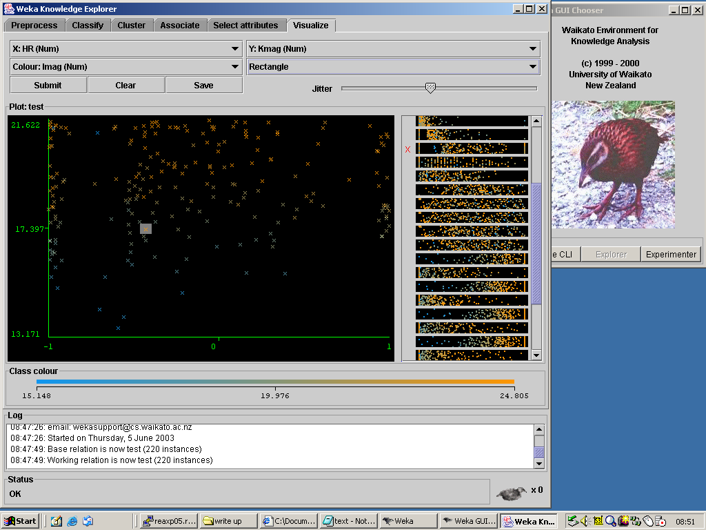
Figure 19. Weka's visualization pane. The right hand portion shows condensed representations
of the scatter plots of all pairs of attributes in the dataset, from which we have selected the
HR vs K magnitude plot to display on the left, with points coloured accordingly to their
I magnitude. An unusually red object has been selected from this plot, as indicated by the shaded
rectangle around it.
To get this we clicked on Weka's Visualize tab, and selected HR and Kmag
respectively from the menus for the X and Y axes. We then chose Imag from
the Colour menu, so that the colour of the points is determined by their I band colour,
as shown in the colour bar at the bottom of the plot. Weka allows us to select an instance from
the dataset, and, in this plot, we have selected a source with an unusually red colour, indicated
by the very faintness of its I band magnitude, given its magnitude at K. The right hand panel of
this window displays the plots of all the pairs of attributes in the data set, and they can be
selected by clicking on them. This is a nice feature, since, whilst they offer very condensed
representations of their data, they do show which plots have structure in them (rather than just
being randomly-populated scatter plots), so one could find the interesting set of plots to view
by scanning over these previews, rather than having to look at each of them in turn.
5.4.3 CViz
The final application that we looked at in this study is CViz, which is a tool for visualizing
clusters in data. It reads in data in CSV format, with the column names in the first row of the
file: we provide the XSL stylesheet to convert from VOTable to CViz format
and the resulting CSV file. CViz is launched by ivoking java on its
.jar file, with additional command line options to set memory allocation, attach the HTML manual, etc,
i.e.
java -cp ctour.jar -mx90M -Dmanual=manual/cviz.html -Dtext=%2 ControlPanel %1
Figure 20 shows a screenshot from CViz:
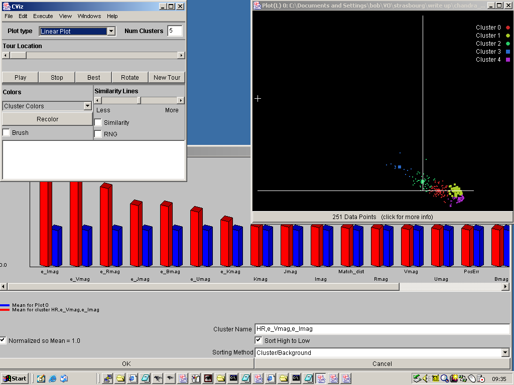
Figure 20. A screenshot showing CViz in action. In the top left is the main CViz window, which
was used to load the dataset and select which attributes to use. The right hand plot shows the
results of CViz's default clustering algorithm run on the data, which generated five clusters.
Clicking on one of them produced the pane at the bottom, which shows the composition of the cluster,
expressed as a comparison of the mean value of each attribute within the cluster members, against
the mean value for the dataset as a whole.
To obtain this after launching CViz we loaded the Chandra/EIS dataset, using the Open Data File
option from the File, and then, from the Select attributes to use pop up which then
appeared, we select the flux/magnitude attributes, plus their uncertainties and the Hardness Ratio
information. CViz then seeks clusters of points in that data space, using its default parameters,
and displays them colour-coded in the right hand pane, in the projection of the data space that most
separates them. Since CViz is designed for handling large amounts of data, it does not plot all the
data points, but, rather, a square symbol to mark the centroid of each cluster, and a representative
sample of points from the cluster, to indicate the dispersion about that centroid. By double clicking
on one of the cluster names in the plot on the right we obtained the panel at the bottom of the
figure, which describes the membership of the cluster in terms of how the mean value of each
attribute differs between the cluster members and the dataset as a whole. As with the Weka clustering
case, we see that CViz's clustering algorithm has basically divided the sample into slices by
optical magnitude, due to the fact that the dispersion in the colours of the objects in the sample
is lower than the dispersion in the overall scaling of their magnitude. So, once again, we should have
applied some normalization to our data before running CViz's clustering algorithm to obtain meaningful
results about possible different source populations.
CViz appears not to offer much in the way of data filtering and manipulation methods, beyond the
selection of which attributes to use, so we would have to have done this before loading the data
into the software.
CViz does have some very nice features. It allows the user to merge the clusters that it has found
automatically, in the case that s/he thinks they have been divided too far, and it can aid that
process by marking the similarity between different clusters. What is particularly nice is its
solution to the problem of how to present the use with multiple scatter plots, created from all
the pairs of attributes in the dataset. It is interesting to compare how our four software
packages do this. In VOPlot, the user would have to select manually the full set of pairs to plot
and look at them one by one, while in Weka, the full set of plots is displayed, in condensed format,
aiding the selection of the interesting ones. Mirage's solution is to display the set of plots one
after the other, with a short pause between each, so that the user can stop the tour, if an
interesting plot appears. This is very nice, but the jerky plotting procedure is a little hard on
the eye, which is something that CViz handles much better. It also plots a tour through the set of
scatter plots of pairs of attributes, but it does so with a smooth animation, so that the cloud of
data points moves smoothly from one plot to the next. This is much easier to watch, and the movement
of the data points in the position for the next plot is suggestive of whether that plot will be
interesting, so it prompts the user to stop the tour and investigate an informative plot more
closely.
5.5 Obtaining more information on X-ray detected EROs
As noted above, Figure 15 suggested a difference in the I-K colour distribution of EROs as a
function of their X-ray hardness ratio, with the reddest EROs amongst the Chandra counterparts
all being very soft X-ray sources.
To investigate the properties of these sources in the high resolution ACS images we
use the ACE web service to measure the sources with SExtractor, and determine whether
they have a dominant optical nuclear component. This was done with the ACE configuration
as shown in Figure 21.
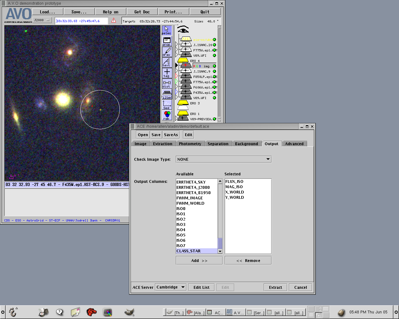
Figure 21. The ACE configuration panel for SExtractor.
Figure 22 shows a RGB image constructed from the ACS F850LP, F775W, and F435W bands, and
overlaid with Chandra error ellipse, and the EIS position (again notice the offset).
This object is clearly extended in the ACS image, and its SExtractor parameters (Low stellarity
index) show there is no dominant nucleus.
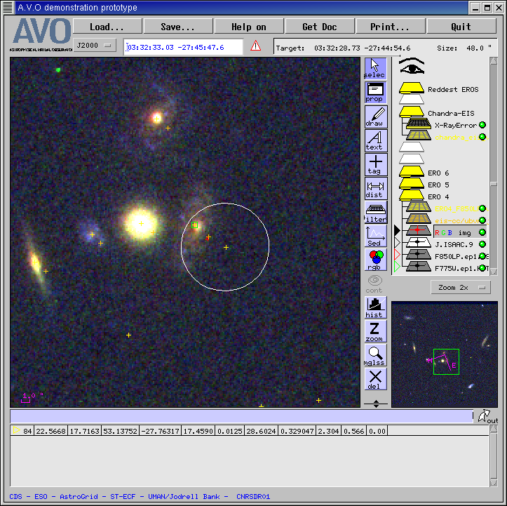
Figure 22. RGB image of one of the most extreme EROs.
6. Discussion and Conclusions
This exercise was primarily intended to address the question "can real science be done with the
first crop of prototype VO tools?", and our answer to that is a positive, if not completely
definitive, "yes, just about". We believe that this exercise has reached the point of
obtaining new science results using existing prototype VO tools, with our needing small workarounds
in only one step where we had to use IDL to generate a VOTable which contained the combined X-ray and optical/NIR
attributes of our cross-matched sources. This we only had to do because of an input formatting problem
in VizieR which has subsequently been tracked down. As such, it is possible to follow this science problem through,
from inception to generation of new results, using existing VO tools, and that is very encouraging.
The VO sceptic might next ask "but couldn't you have done this more easily using other, non-VO
tools?", to which the honest answer is "no, probably not". It is true that the ERO
selection and the generation of the various figures above plotting attributes against each other, etc,
could have been readily produced in IDL, say, but we have used a lot of different data sets in this
exercise, and an IDL programmer would have had to have figured out the data formats and structures
of each before being able to load them: the level of interoperability between data sources present
in this first generation of VO tools is already a boon to astronomical research.
One thing that is clear from this exercise is that there are a number of non-astronomical tools
available which could prove very valuable for the exploration of the multi-dimensional datasets
of attributes produced by cross-matching different astronomical catalogues. We barely scratched
the surface of what can be done with general data mining packages, such as Weka, and these are
likely to become important as the VO develops, and it is crucial that the VO infrastructure
supports their use; for example, through the availability of the XSLT transformations needed
to convert VOTable into their specific data formats, so that such tools can be readily use as
part of a VO data analysis workflow. It was clear, however, even from our brief foray into their
use, that such tools cannot be regarded as black boxes, to be used blindly on any astronomical
dataset. We found that we did not obtain very enlightening results from running Weka and CViz
simply because we had not thought properly about what data to give them, while, at a more
general level, we would have to understand the myriad algorithms and options offered by such
tools before we could start to use them effectively.
Our exercise did identify a number of gaps in the current prototype VO toolkit:
- Cross-match tool: Simple positional cross-matching, as we performed here, can
be done in VizieR, when at least one of the pair of catalogues involved is held there,
but there is clearly a need for a more sophisticated association tool that
can match sources using more than proximity. In the general case, one would want to encode
prior knowledge about the source populations involved into some sort of likelihood ratio
technique (or equivalent), so that one could choose between multiple counterparts with
acceptable positional offsets. In our example, we had several cases of a Chandra source
which had more than one EIS object within its error circle, and we simply took the closest
match, because we had no other information to use in choosing between the candidates. In
situations such as this, it would be advantageous for the cross-match tool to return attributes
for a number of possible associations, along with a figure of merit (e.g. positional offset
in our case, or some probability, more generally) so that the astronomer can make the
choice for herself.
- VOTAble editor/viewer: One of the problems that we came across trying to use
the non-astronomical tools to analyse our data was that we didn't have exactly the correct
attributes to read into the tool (e.g. magnitudes, not colours) nor did the tool offer the
functionality required to create them. It would be very useful to have some sort of editor
with which one could inspect a VOTable in tabular form and also generate additional columns,
select rows with predicates on existing columns, etc, as might be required. VOPlot's virtual
column and filter mechanism do this, but a drawback is that one is not able to
export modified VOTables after these functions have been applied. The developmental
version of VOPlot does however have a VOTable export facility.
- Data transformation tools/toolkits: One of the main benefits of using an XML data
format, like VOTable, is the ease with which XSLT can be used to transform data from VOTable
to the formats required by other tools: this is a great bonus for the VO, as it opens up
a wealth of useful existing tools produced outwith astronomy, of which Mirage, Weka and
CViz are but three examples. The challenge for the VO, then, is to help astronomers use
these tools, which requires the availability of data transformation services. Whilst it
would be unreasonable to expect the VO to offer the services necessary to transform VOTable
into the formats used by every single data exploration tool that any astronomer could
possibly want to use, it is feasible to imagine their being services covering a subset of
the most powerful tools, together with a toolkit to help astronomers produce the XSLT
scripts needed for use of tools not in that subset.
- Workflow/scripting: A general VO requirement will be to be able to store and
reapply parameterised workflows. For example, in Section 5.5 we had to obtain additional
information for a list of sources we had identified as being interesting. For each source,
this involved executing a series of steps, using Aladin and ACE, and this series had to
be executed for each source in turn. Clearly, it would be highly desirable to be able to
generate a workflow by running an analysis procedure once manually, and then being able
to run it for a series of input parameter values (e.g. source positions, in our example).
This clearly requires analysis tools that can be run in a scripted manner, rather than
just interactively.
- Postage stamp tool: A concrete example of a workflow that is often repeated
many times in the execution of a science problem is the generation of postage stamp
images of sources. It would be very useful for image servers to offer a mode in which
the user could supply a list of source positions and have postage stamp cut out images
returned and displayed. Some image servers support this already, but it would appear
to be a general requirement.
Acknowledgement:
Bob Mann gratefully acknowledges the award of a Professeur invité position at the
Université Louis Pasteur, Strasbourg during the period within which this work was
undertaken.