
MPMP Displays Using Trellis Display
Visualization tools are vital for analyzing a very large traffic
database. Analytic visualization tools support model development.
One issue is screen real estate. Because Internet databases are
large and the structure is complex, we
must accept the notion that single displays need to cover tens and perhaps
hundreds of pages with many panels on each page. Data visualization is
often limited to a display of a set of data that can be placed all at
once in our visual field. So it can be shocking at first to contemplate
looking at so many pages. But using the structure of
trellis display,
a visualization system available in S/S-PLUS, it
is easy to generate many pages. And using a document
viewer, it is possible to learn a great deal about Internet traffic data
from these multipage, multipanel, or MPMP, displays.
One Example: The Inter-Arrival Plot
This is a trellis display with one page and two panels; it displays the
HTTP start times for 2 of 10704 blocks of data.
It was immensely informative
for modeling the start times to see such displays for hundreds of blocks.
And the only practical medium to communicate these MPMP displays is our
medium of study, the Internet.
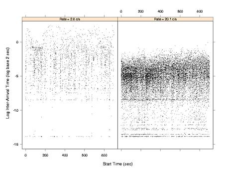
Click here for the postscript file of the plot.
The left panel of the figure, an inter-arrival plot , displays the 2515 HTTP start times for one block, 7:45 a.m. to 8:00 a.m. on 12/11/98. Let s(k) for k = 1 to 2515 be the start times, and let t(k) = s(k) - s(k-1) for k = 2 to 2515 be the inter-arrival times. On the plot, l(k) = log base 2 t(k) is graphed against s(k). The log on the vertical scale is vital because inter-arrivals can vary over 16 powers of 2, a factor of about 64000, and small intervals are as important as large ones; so the vertical scale provides the requisite resolution to see this variation. The horizontal scale, however, conveys arrivals and inter-arrivals on the original scale. The connection rate over this block is 2.8 connections per second (c/s). The right panel of Figure 1 is an inter-arrival plot for the block 12:15 p.m. to 12:30 p.m. on the same day; the connection rate is 20.1 c/s.
Both panels show discreteness on the vertical scale, inter-arrivals piling up at a few values. This is a network effect, a small delay; each accumulation point is a time equal to the time it takes to process a packet in the network. For example, suppose two SYN packets are back to back, which happens a small fraction of the time. The inter-arrival time is the time it takes to read the first packet, which is the packet size times the wire speed; at the time of collection the speed was 10 megabits/sec.
The HTTP start times are a superposition point process. Each user generates an HTTP start time point process on the wire, and the aggregate start time process is the superposition of the user point processes. In the figure, the connection rate is greater in the left panel than in the right because there are more users browsing the Web from 12:15 p.m. to 12:30 p.m. than from 7:45 a.m. to 8:00 a.m. In other words, the number of superposed processes in the later period is greater. The different amounts of superposition dramatically affect the statistical properties of the inter-arrival times. In the bottom panel, the data form distinct, narrow vertical bands for which the $l(k)$ range from about -8 log sec to about -2 log sec. The bands are bursts of connections caused by single clicks of individual users. The number of connections in such bursts can be large because the number of embedded files has a distribution with a long upper tail. In the top panel, the bursty behavior has disappeared. Because the connection rate is much higher, the SYNs of more users intermingle, and the behavior of individual users is broken up. For both panels, the l(k) sequence exhibits long-range dependence, a slowly decaying positive autocorrelation function. But for the left panel, the autocorrelation is much less than that for the right panel. For both panels, the marginal empirical distribution of the t(k) is well approximated by a Weibull (except for the discreteness), with a shape parameter less than 1, the shape for an exponential. But for the left panel, the value of the shape is much greater than that for the right.
The analysis of the HTTP start times produced the following conclusions. The marginal distribution of the t(k) is approximately Weibull with shape less than 1, and as the connection rate increases, the shape tends toward 1. The change in the distribution over the 10704 blocks is large; the estimate of the shape ranges from about 0.4 to 0.9. The autocorrelation of the l(k) is described by an exceedingly simple model with two parameters: white noise plus a long-range persistent time series. The two parameters are the variances of the two series. As the connection rate increases, the variance of the persistent series tends toward zero, and the l(k) tend toward independence. The change in the autocorrelation function over the blocks is large; the fraction of the variance of l(k) accounted for by the persistent series ranges from about 0.5 to 0.1.
The inter-arrival plot and many other visualization tools were essential to discovering these phenomena.