
The original implementation was written by Rick Becker, Linda Clark, and Diane Lambert.
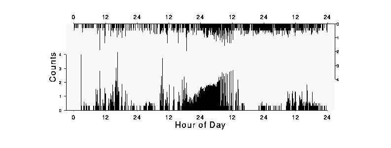
The coordinate axes for the y series are shown by the left vertical axis and bottom horizontal time scale, while the coordinate axes for the y.top series are shown by the right vertical axis and the top horizontal time scale. The y and y.top horizontal axes are identical, but showing both makes it as easy to find time points for the y.top series as it is to find time points for the y series.
The y and y.top vertical axes are different, though.
The y vertical axis increases from bottom to top, as usual,
but the y.top vertical axis is opposed in the sense that
it increases from top to bottom.
The vertical axes can overlap ,
so that the y and y.top
series can share part of the plotting region if the data so warrants.
Because the extreme values from y and y.top
in Figure 1 do not occur simultaneously,
re-using the plotting region does not destroy information. It only puts the
two series closer together, saving space and making them easier to compare
visually.
x:	x values for the lower time series.
y:	y values for the lower portion of the plot.
x.top:	x values for the upper time series.
y.top:	y values for the upper portion of the plot.
overlap:   percent of overlap. For example, 100% overlap means the entire
	vertical plotting region is shared by the lower and upper value.
	0% overlap means there will be no overlap.
xaxis.at:        where xaxis ticks will be placed.
xaxis.lab:       labels for those ticks.
yaxis.at:        where left yaxis ticks will be placed.
yaxis.lab:       labels for those ticks.
xlab:		xaxis label.
ylab:		yaxis label.
Figure 1 was produced by this call:
cave.plot(digtime, y, digtime, y.top, overlap=50,
        xaxis.at=seq(0,96,12),
        xaxis.lab=c(0,rep(c(12,24),4)),
        yaxis.at=0:4, yaxis.lab=as.character(0:4),
        xlab="Hour of Day", ylab="Counts")
The data are 2884 counts of air particles at two locations (y and
y.top) taken over 4 days. The x values are number of hours from the
start of counting, so they range from 0 to 96.
Since the upper y values are mostly smaller than the lower,
choosing overlap=50 increases the vertical range of the plot by 50%,
allowing partial reuse of the plotting region by the lower and upper
portions of the plot while still leaving most of the data visible. Below
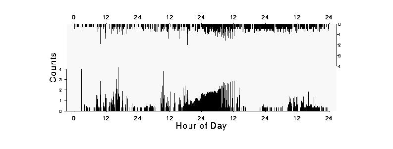
is the same plot with overlap=0 -- as you can see, there is a lot of
wasted space and the segments are much shorter.
 Ticks for the xaxis were chosen to be every 12 hours, labeled simply
as 12 and 24.
Left axis labels are at 0 to 4, the range of the data.
The right axis will have the same axis labels, appropriately reversed.
You may view a postscript version of the paper: