Help for irregular LDPC code design demo.
This is a demo version of the irregular low-density parity-check
(LDPC) code
optimizer for additive white Gaussian noise (AWGN) channel with
binary antipodal signaling.
This program does the optimization for a given rate and complexity
assuming 1) infinite block length, 2) random interleaver and 3)
Gaussian approximation for the posterior
log likelihood densities. For more general theory that does not
rely on the Gaussian approximation, see
Design of Provably Good Low-Density Parity Check Codes by Thomas
Richardson, Amin Shokrollahi and Rüdiger Urbanke.
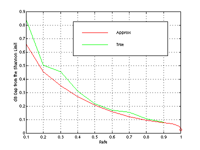
The following graph shows the performance of
the irregular LDPC codes designed by this program for AWGN channel
with binary antipodal signaling,
where the red curve shows the dB gap calculated using Gaussian
approximation
and the green curve is the true dB gap.
Explanation of inputs:
- Rate: Rate of the code. Since the Gaussian approximation does not
work very well if the rate is less than 0.1 and since some special
care is
needed when the rate is very high ( > 0.99), this should be
between
0.1 and 0.99 for this demo version.
Rate can be also specified as a fraction.
- Left degree sequence: This sequence is used to specify
the set of fractions of edges that belong to certain degree nodes
on the left hand side (i.e. variable nodes) of the LDPC codes.
The complexity of the code can be controlled by limiting the
maximum
degree for the variable nodes.
Users can specify either the maximum degree or more generally
a set of allowed degrees.
Maximum degree in either case is limited to 20, since the
Gaussian
approximation does not work well beyond that.
- Average right degree: This program does not try to optimize the
degree sequence for check nodes, since this sequence tends to
be concentrated anyway. You may want to try several values for
this
item to optimize the code for a given rate and a maximum left
degree.
The following table shows some values of the average right degree
that maximize the threshold predicted by the
approximation. These values were used
to generate the above figure
for rate = 0.1, ... 0.9 when the maximum left degree was 20.
| Rate | average right degree |
|---|
| 0.1 | 3.55 |
| 0.2 | 4.61 |
| 0.3 | 5.81 |
| 0.4 | 7.03 |
| 0.5 | 8.75 |
| 0.6 | 11.44 |
| 0.7 | 17.56 |
| 0.8 | 26.5 |
| 0.9 | 54 |
Warning: If suboptimal values of the average right degree are
used,
then in some cases the actual threshold is much worse than the
threshold predicted by the approximation.
Explanation of outputs:
- Capacity: This is the channel capacity in terms of the noise
standard deviation (sigma) and Eb/N0 for a given rate.
- Approximate threshold: This is the capacity achievable by the
designed code in terms of the noise standard deviation (sigma)
and Eb/N0. Since this calculation is based on approximation,
true value would be slightly different. See the above graph
for some examples.
- Gap from the Shannon limit: This is the dB gap from the Shannon
limit
for the designed code.
- Degree sequence for variable nodes: This is the degree sequence
for variable nodes in edge perspective (i.e. L[n] is the
fraction of edges
that belong to degree-n variable nodes).
- Degree sequence for check nodes: This is also in edge
perspective.
- Degree sequence for variable nodes (node perspective): This is
the degree sequence
for variable nodes in node perspective (i.e. L[n] is the
fraction of nodes that have degree n).
- Degree sequence for check nodes (node perspective): Same as
above
but for check nodes.
Return to demo
by Sae-Young
Chung, Rüdiger
L. Urbanke, Thomas J.
Richardson
Questions or comments? sychung@mit.edu, ruediger@lucent.com, tjr@lucent.com
Last modified on Wednesday August 25, 1999